Shapeoko 2 calibration runs

Background

After some issues with accuracy drilling holes in PCBs and concern about backlash with the GT2 belt drive that makes some real machinists roll their eyes, it was time to do some initial calibration investigation.

Bill P brought in a USB microscope for such use some time ago, and at the great personal cost of a virus infection, Daniil found a good driver for it.  We put a viewer and the driver on the SO laptop and got pictures!  The lines scribed on my dear old 6″ Craftsman vernier caliper served as a good linear calibration reference.

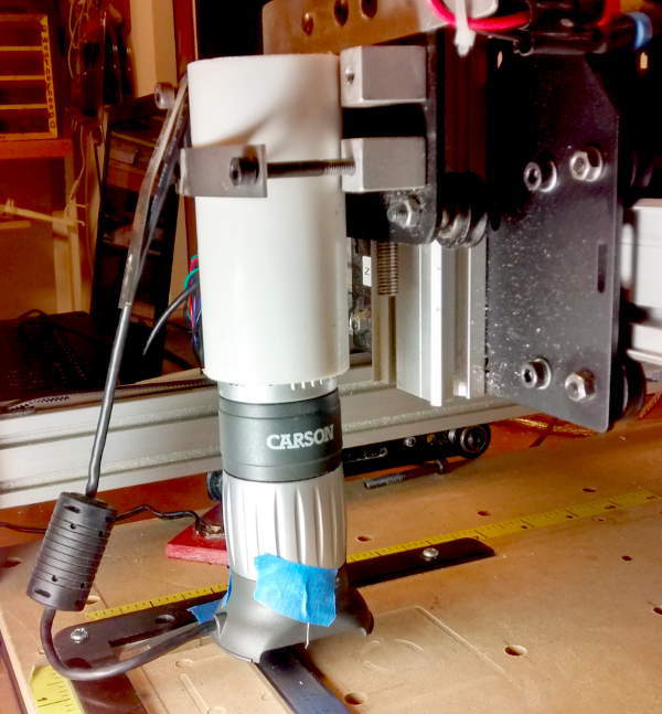The microscope friction fit perfectly in a scrap of PVC pipe we clamped in place of the spindle.  As a “crosshair”, we taped a .007″ strand of hookup wire across the bottom of the ‘scope.  We found we needed more light than the little built-in LEDs provided when we zoomed in like we wanted, so we clamped a reflector lamp near by to provide that light.  Here’s the whole setup.

I had to disassemble the movable jaw from the caliper to let the ‘scope get close enough.  That’s the first time it’s been off in the 50+ years (!) I’ve 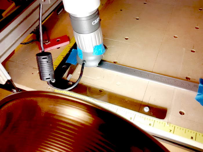had that caliper.  It went back together perfectly after the testing.

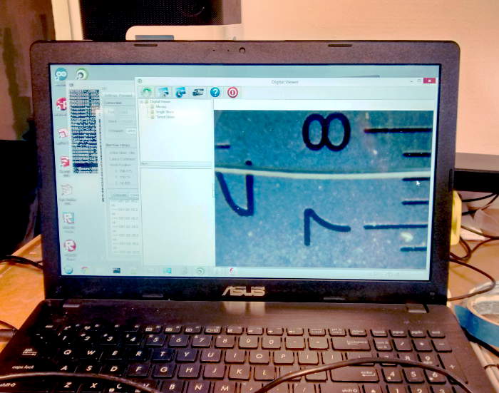The image from the ‘scope was very nice.  The white stripe is the crosshair wire.  A finer wire would have been even better.  The marks shown are spaced at 0.025″.

The calibration runs

As soon as we started playing using UGS jog controls to move the gantry, the backlash was clearly visible.  We decided to record observations every 0.2″ for the 6″ of movement the caliper allowed, going first one direction, then coming back the other way.  Based on the informal backlash observations, we were careful to approach the initial mark going in the right direction.  We did a run each way in X, then moved the caliper and did another pair in Y.

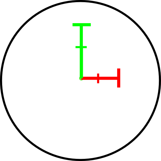
Since the 0.2″ steps should always have fallen exactly on a (long) etch line, we recorded the error at each point.  We started out using “wire diameters” as the unit of measure, but as some errors became larger, we switched to eyeball estimates based on the 0.025″ line spacing.  The red lines are X, green are Y. 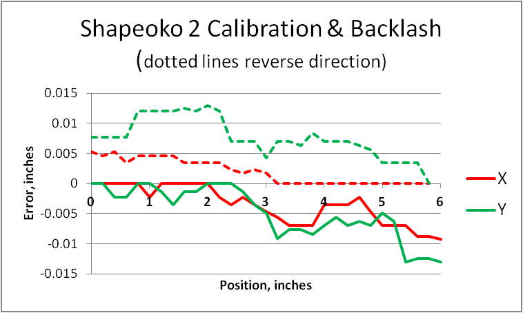 The dotted lines are coming back in the reverse direction (toward X|Y=0).  Observations:

• Especially in X (solid red), the first couple of inches of steps were right on – and then got worse.  Similar patterns in all runs suggest some belt stretch.  Of course the X and Y stretch happening about the same place is coincidence.  (And no, I don’t think my caliper is stretched at that point.)  The fact that there’s a clear overall worsening of error with larger displacements from 0,0 supports belt strech.
• Backlash is completely obvious.  Taking difference between average of observed values going forward and backward, average backlash on X is 0.0055″; on Y 0.0125″.  Similarly with max values, the worst case backlash on X is 0.0146″; on Y it’s 0.026″.  I wonder how new belts would behave.
• In terms of the real-world task requiring the highest precision we’ve asked of the SO2 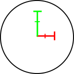so far – drilling PCBs – the results are “interesting”.  With holes from my favorite #64 drill at about 0.039″ diameter (black circle), the average absolute error in X (red) of about 0.0028″ and even worst error of 0.0053″ aren’t bad at all.  The Y (green) average error of 0.0062″ isn’t too bad, but the worst case error of 0.013″ is a third of a hole diameter – worth some concern.  (There must be a better way to present this visually.)

Of course the backlash observed with the microscope involved no loading of the gantry.  If we tried isolation milling of PCBs, adding some load deformation to that backlash might result in requiring much larger features (like traces) than we’d like.  Of course it would be much poorer than the photo PCB process, but at least it would involve no tool-rusting vapors!

Possible next steps

Another possible calibration approach would use an optical belt scavenged from a printer or scanner.  Its 350mm length is plenty to observe the full 200mm or so of travel on each axis.  From a good graticule on a loupe, I believe the lines are 1/180″ (0.00555…”).  A laser diode scavenged from one of the laser levels and some scrap lens assembly may focus the beam to small enough to resolve the lines at the focal point.  While the resolution isn’t as good as the microscope, with an Arduino sending gcode steps and counting bars, it could provide an automated tool with lots more points and no human error.

Given the possibility of stretched belts and Inventables price of $2/foot for 6mm G2 belting, a $10 investment in all new belts probably makes sense.  And with automated calibration runs of old and new belts, it would provide an interesting observation experiment as well as a probably a more accurate Shapeoko.